8. Embedding
In the previous chapter we looked at some tools for examining the ways that individuals are connected, and the distances between them. In this chapter we will look at the same issue of connection. This time, though, our focus is the social structure, rather than the individual. That is, we will adopt a more "macro" perspective that focuses on the structures within which individual actors are embedded.
The "top down" perspective we'll follow in this chapter seeks to understand and describe whole populations by the "texture" of the relations that constrain its individual members. Imagine one society in which extended kin groups live in separate villages at considerable distances from one another. Most "texture" of the society will be one in which individuals have strong ties to relatively small numbers of others in local "clusters." Compare this to a society where a large portion of the population lives in a single large city. Here, the "texture" of social relations is quite different -- individuals may be embedded in smaller nuclear families of mating relations, but have diverse ties to neighbors, friends, co-workers, and others.
Social network analysts have developed a number of tools for conceptualizing and indexing the variations in the kinds of structures that characterize populations. In this chapter, we'll examine a few of these tools.
The smallest social structure in which an individual can be embedded is a dyad (that is, a pair of actors). For binary ties (present or absent), there are two possibilities for each pair in the population - either they have a tie, or they don't. We can characterize the whole population in terms of the prevalence of these dyadic "structures." This is what the density measure does.
If we are considering a directed relation (A might like B, but B might not like A), there are three kinds of dyads (no tie, one likes the other but not vice versa, or both like the other). The extent to which a population is characterized by "reciprocated" ties (those where each directs a tie to the other) may tell us about the degree of cohesion, trust, and social capital that is present.
The smallest social structure that has the true character of a "society" is the triad - any "triple" {A, B, C} of actors. Such a structure "embeds" dyadic relations in a structure where "other" is present along with "ego" and "alter." The analysis of triads, and the prevalence of different types of triads in populations has been a staple of sociometry and social network analysis. In (directed) triads, we can see the emergence of tendencies toward equilibrium and consistency -- institutionalization -- of social structures (balance and transitivity). Triads are also the simplest structures in which we can see the emergence of hierarchy.
Most of the time, most people interact with a fairly small set of others, many of whom know one another. The extent of local "clustering" in populations can be quite informative about the texture of everyday life. Actors are also embedded in "categorical social units" or "sub-populations" defined either by shared attributes or shared membership. The extent to which these sub-populations are open or closed - the extent to which most individuals have most of their ties lives within the boundaries of these groups - may be a telling dimension of social structure.
There are many approaches to characterizing the extent and form of "embedding" of actors in populations. There is no one "right" way of indexing the degree of embedding in a population that will be effective for all analytic purposes. There are, however, some very interesting and often useful approaches that you may wish to explore.
If we are comparing two populations, and we note that there are many actors in one that are not connected to any other ("isolates"), and in the other population most actors are embedded in at least one dyad -- we would likely conclude that social life is very different in the two populations.
Measuring the density of a network gives us a ready index of the degree of dyadic connection in a population. For binary data, density is simply the ratio of the number of adjacencies that are present divided by the number of pairs - what proportion of all possible dyadic connections are actually present. If we have measured the ties among actors with values (strengths, closeness, probabilities, etc.) density is usually defined as the sum of the values of all ties divided by the number of possible ties. That is, with valued data, density is usually defined as the average strength of ties across all possible (not all actual) ties. Where the data are symmetric or un-directed, density is calculated relative to the number of unique pairs ((n*n-1)/2); where the data are directed, density is calculated across the total number of pairs.
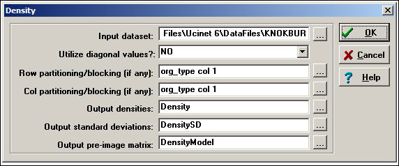
Network>Cohesion>Density is a useful tool for calculating the density of whole populations, or of partitions. A typical dialog is shown in figure 8.1.
Figure 8.1. Dialog of Network>Cohesion>Density

In this dialog, we are again examining the Knoke information tie network. We have used an attribute or partition to divide the cases into three sub-populations (governmental agencies, non-governmental generalist, and welfare specialists) so that we can see the amount of connection within and between groups. This is done by creating a separate attribute data file (or a column in such a file), with the same row labels, and scores for each case on the "partitioning" variable. Partitioning is not necessary to calculate density. The results of the analysis are shown in figure 8.2.
Figure 8.2. Density of three sub-populations in Knoke information network
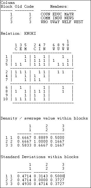
After providing a map of the partitioning, a blocked (partitioned) matrix is provided showing the values of the connections between each pair of actors. Next, the within-block densities are presented. The density in the 1,1 block is .6667. That is, of the six possible directed ties among actors 1, 3, and 5, four are actually present (we have ignored the diagonal -- which is the most common approach). We can see that the three sub-populations appear to have some differences. Governmental generalists (block 1) have quite dense in and out ties to one another, and to the other populations; non-government generalists (block 2) have out-ties among themselves and with block 1, and have high densities of in-ties with all three sub-populations. The welfare specialists have high density of information sending to the other two blocks (but not within their block), and receive more input from governmental than from non-governmental organizations.
The extent to which these simple characterizations of blocks characterize all the individuals within those blocks -- essentially the validity of the blocking -- can be assessed by looking at the standard deviations within the partitions. The standard deviations measure the lack of homogeneity within the partition, or the extent to which the actors vary.
A social structure in which individuals were highly clustered would display a pattern of high densities on the diagonal, and low densities elsewhere.
With symmetric dyadic data, two actors are either connected, or they are not. Density tells up pretty much all there is to know.
With directed data, there are four possible dyadic relationships: A and B are not connected, A sends to B, B sends to A, or A and B send to each other. A common interest in looking at directed dyadic relationships is the extent to which ties are reciprocated. Some theorists feel that there is an equilibrium tendency toward dyadic relationships to be either null or reciprocated, and that asymmetric ties may be unstable. A network that has a predominance of null or reciprocated ties over asymmetric connections may be a more "equal" or "stable" network than one with a predominance of asymmetric connections (which might be more of a hierarchy).
There are (at least) two different approaches to indexing the degree of reciprocity in a population. Consider the very simple network shown in figure 8.3. Actors A and B have reciprocated ties, actors B and C have a non-reciprocated tie, and actors A and C have no tie.
Figure 8.3. Definitions of reciprocity
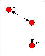
What is the prevalence of reciprocity in this network? One approach is to focus on the dyads, and ask what proportion of pairs have a reciprocated tie between them? This would yield one such tie for three possible pairs (AB, AC, BC), or a reciprocity rate of .333. More commonly, analysts are concerned with the ratio of the number of pairs with a reciprocated tie relative to the number of pairs with any tie. In large populations, usually most actors have no direct ties to most other actors, and it may be more sensible to focus on the degree of reciprocity among pairs that have any ties. In our simple example, this would yield one reciprocated pair divided by two tied pairs, or a reciprocity rate of .500. The method just described is called the dyad method in Network>Cohesion>Reciprocity.
Rather than focusing on actors, we could focus on relations. We could ask, what percentage of all possible ties (or "arcs" of the directed graph) are parts of reciprocated structures? Here, two such ties (A to B and B to A) are a reciprocated structure among the six possible ties (AB, BA, AC, CA, BC, CA) or a reciprocity of .333. Analysts usually focus, instead, on the number of ties that are involved in reciprocal relations relative to the total number of actual ties (not possible ties). Here, this definition would give us 2 / 3 or .667. This approach is called the arc method in Network>Cohesion>Reciprocity. Here's a typical dialog for using this tool.
Figure 8.4. Dialog for Network>Network Properties>Reciprocity
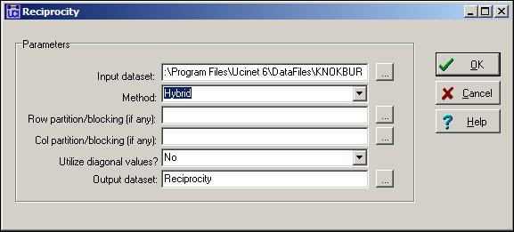
We've specified the "hybrid" method (the default) which is the same as the dyad approach. Note that it is possible to block or partition the data by some pre-defined attribute (like in the density example above) to examine the degree of reciprocity within and between sub-populations. Figure 8.5 shows the results for the Knoke information network.
Figure 8.5. Reciprocity in the Knoke information network

We see that, of all all pairs of actors that have any connection, 53% of the pairs have a reciprocated connection. This is neither "high" nor "low" in itself" but does seem to suggest a considerable degree of institutionalized horizontal connection within this organizational population.
The alternative method of "arc" reciprocity (not shown here) yield a result of .6939. That is, of all the relations in the graph, 69% are parts of reciprocated ties.
Small group theorists argue that many of the most interesting and basic questions of social structure arise with regard to triads. Triads allow for a much wider range of possible sets of relations.
With un-directed data, there are four possible types of triadic relations (no ties, one tie, two ties, or all three ties). Counts of the relative prevalence of these four types of relations across all possible triples (that is a "triad census") can give a good sense of the extent to which a population is characterized by "isolation," "couples only," "structural holes" (i.e. where one actor is connected to two others, who are not connected to each other), or "clusters." UCINET does not have a routine for conducting triad censuses (see Pajek, which does).
With directed data, there are actually 16 possible types of relations among 3 actors), including relationships that exhibit hierarchy, equality, and the formation of exclusive groups (e.g. where two actors connect, and exclude the third). Thus, small group researchers suggest, all of the really fundamental forms of social relationships can be observed in triads. Because of this interest, we may wish to conduct a "triad census" for each actor, and for the network as a whole (again, see Pajek).
In particular, we may be interested in the proportion of triads that are "transitive" (that is, display a type of balance where, if A directs a tie to B, and B directs a tie to C, then A also directs a tie to C). Such transitive or balanced triads are argued by some theorists to be the "equilibrium" or natural state toward which triadic relationships tend (not all theorists would agree!).
Of the 16 possible types of directed triads, six involve zero, one, or two relations -- and can't display transitivity because there are not enough ties to do so. One type with 3 relations (AB, BC, CB) does not have any ordered triples (AB, BC) and hence can't display transitivity. In three more types of triads, there are ordered triples (AB, BC) but the relation between A and C is not transitive. The remaining types of triads display varying degrees of transitivity.
UCINET does not have extensive algorithms for examining full triad censuses and building more complex models based on them (e.g. balance, clusterability, ranked clusters). A more extended treatment of this approach, with supporting software is available from Pajek. Nonetheless, the Network>Cohesion>Transitivity algorithms in UCINET offer some interesting and flexible approaches to characterizing the transitivity of triads in populations. A typical dialog is shown in figure 8.6.
Figure 8.6. Dialog of Network>Cohesion>Transitivity
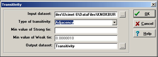
The Knoke information network is a binary, directed graph. For data of this type, the default definition of transitivity (i.e. "Adjacency") is a reasonable approach. This means that we will count the number of times that, if we see AB and BC, we also see AC.
Network>Cohesion>Transitivity also provides some alternative definitions of what it means for a triad to be transitive which are useful for valued data.
A strong transitivity is one in which there are connections AB, BC, and AC, and the connection AC is stronger than the Min value of Strong tie. A weak transitivity is one in which there are connections AB, BC and AC, and AC; the value of AC is less than the threshold for a strong tie, but greater than the threshold Min value of Weak tie.
Two other methods are also available. A Euclidean transitivity is defined as a case where AB, BC, and AC are present, and AC has a value less than the sum of AB + BC. A Stochastic transitivity is defined as the case where AB, BC, and AC are present, and AC is less than the produce AB*BC.
Figure 8.7. Transitivity results for Knoke information network

After performing a census of all possible triads, Network>Cohesion>Transitivity reports that it finds 146 transitive (directed) triples. That is, there are 146 cases where, if AB and BC are present, then AC is also present. There are a number of different ways in which we could try to norm this count so that it becomes more meaningful. One approach is to divide the number of transitive triads by the total number of triads of all kinds (720). This shows that 20.28% of all triads are transitive. Perhaps more meaningful is to norm the number of transitive triads by the number of cases where a single link could complete the triad. That is, norm the number of {AB, BC, AC} triads by the number of {AB, BC, anything} triads. Seen in this way, about 2/3 or all relations that could easily be transitive, actually are.
Watts (1999) and many others have noted that in large, real-world networks (of all kinds of things) there is often a structural pattern that seems somewhat paradoxical.
On one hand, in many large networks (like, for example, the Internet) the average geodesic distance between any two nodes is relatively short. The "6-degrees" of distance phenomenon is an example of this. So, most of the nodes in even very large networks may be fairly close to one another. The average distance between pairs of actors in large empirical networks are often much shorter than in random graphs of the same size.
On the other hand, most actors live in local neighborhoods where most others are also connected to one another. That is, in most large networks, a very large proportion of the total number of ties are highly "clustered" into local neighborhoods. That is, the density in local neighborhoods of large graphs tend to be much higher than we would expect for a random graph of the same size.
Most of the people we know may also know one another -- seeming to locate us in a very narrow social world. Yet, at the same time, we can be at quite short distances to vast numbers of people that we don't know at all. The "small world" phenomena -- a combination of short average path lengths over the entire graph, coupled with a strong degree of "clique-like" local neighborhoods -- seems to have evolved independently in many large networks.
We've already discussed one part of this phenomenon. The average geodesic distance between all actors in a graph gets at the idea of how close actors are together. The other part of the phenomenon is the tendency towards dense local neighborhoods, or what is now thought of as "clustering."
One common way of measuring the extent to which a graph displays clustering is to examine the local neighborhood of an actor (that is, all the actors who are directly connected to ego), and to calculate the density in this neighborhood (leaving out ego). After doing this for all actors in the whole network, we can characterize the degree of clustering as an average of all the neighborhoods.
Figure 8.8 shows the output of Network>Cohesion>Clustering Coefficient as applied to the Knoke information network.
Figure 8.8. Network>Cohesion>Clustering Coefficient of Knoke information network

Two alternative measures are presented. The "overall" graph clustering coefficient is simply the average of the densities of the neighborhoods of all of the actors. The "weighted" version gives weight to the neighborhood densities proportional to their size; that is, actors with larger neighborhoods get more weight in computing the average density. Since larger graphs are generally (but not necessarily) less dense than smaller ones, the weighted average neighborhood density (or clustering coefficient) is usually less than the un-weighted version. In our example, we see that all of the actors are surrounded by local neighborhoods that are fairly dense -- our organizations can be seen as embedded in dense local neighborhoods to a fairly high degree. Lest we over-interpret, we must remember that the overall density of the entire graph in this population is rather high (.54). So, the density of local neighborhoods is not really much higher than the density of the whole graph. In assessing the degree of clustering, it is usually wise to compare the cluster coefficient to the overall density.
We can also examine the densities of the neighborhoods of each actor, as is shown in figure 8.9.
Figure 8.9. Node level clustering coefficients for Knoke information network
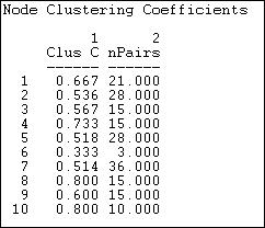
The sizes of each actor's neighborhood is reflected in the number of pairs of actors in it. Actor 6, for example has three neighbors, and hence three possible ties. Of these, only one is present -- so actor 6 is not highly clustered. Actor 8, on the other hand, is in a slightly larger neighborhood (6 neighbors, and hence 15 pairs of neighbors), but 80% of all the possible ties among these neighbors are present. Actors 8 and 10 are embedded in highly clustered neighborhoods.
Actors may be embedded in macro-structures, as well as in dyads, triads, and neighborhoods. Some macro-structures are social agents (like voluntary and formal organizations); some macro-structures are categorical units (like gender and ethnic groups). To understand the "texture" of the "social fabric" we might want to index the extent to which these macro-structures "cluster" the interaction patterns of individuals who fall within them.
Krackhardt and Stern (1988) developed a very simple and useful measure of the group embedding based on comparing the numbers of ties within groups and between groups. The E-I (external - internal) index takes the number of ties of group members to outsiders, subtracts the number of ties to other group members, and divides by the total number of ties. The resulting index ranges from -1 (all ties are internal to the group) to +1 (all ties are external to the group). Since this measure is concerned with any connection between members, the directions of ties are ignored (i.e. either a out-tie or an in-tie constitutes a tie between two actors).
The E-I index can be applied at three levels: the entire population, each group, and each individual. That is, the network as a whole (all the groups) can be characterized in terms of the bounded-ness and closure of its sub-populations. We can also examine variation across the groups in their degree of closure; and, each individual can be seen as more or less embedded in their group.
Here's a sample of the dialog with Network>Cohesion>E-I Index in which we examine the Knoke information network that has been partitioned according to the attribute of organizational type (group 1 = governmental generalists, group 2 = non-governmental generalists, group 3 = welfare specialists).
Figure 8.10. Dialog of Network>Cohesion>E-I Index

The range of possible values of the E-I index is restricted by the number of groups, relative group sizes, and total number of ties in a graph. Often this range restriction is quite severe, so it is important to re-scale the coefficient to range between the maximum possible degree of "external-ness" (+1) and the maximum possible degree of "internal-ness." As Blau and others have noted, the relative sizes of sub-populations have dramatic consequences for the degree of internal and external contacts, even when individuals may choose contacts at random.
To assess whether a give E-I index value is significantly different that what would be expected by random mixing (i.e. no preference for within or without group ties by group members), a permutation test is performed by Network>Cohesion>E-I Index. A large number of trials are run in which the blocking of groups is maintained, and the overall density of ties is maintained, but the actual ties are randomly distributed. From a large number of trials (the default is 5000), a sampling distribution of the numbers of internal and external ties -- under the assumption that ties are randomly distributed -- can be calculated. This sampling distribution can then be used to assess the frequency with which the observed result would occur by sampling from a population in which ties were randomly distributed.
Let's look first at the results for the graph as a whole, in figure 8.11.
Figure 8.11. E-I index output for the Knoke information network - whole network
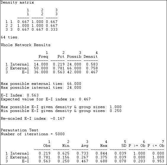
The observed block densities are presented first. Since any tie (in or out) is regarded as a tie, the densities in this example are quite high. The densities off the main diagonal (out-group ties) appear to be slightly more prevalent than the densities on the main diagonal (in-group ties).
Next, we see the numbers of internal ties (14, or 22%) and external ties (50, or 78%) that yield a raw (not rescaled) E-I index of +.563. That is, a preponderance of external over internal ties for the graph as a whole. Also shown are the maximum possible numbers of internal and external ties given the group sizes and density. Note that, due to these constraints, the result of a preponderance of external ties is not unexpected -- under a random distribution, the E-I index would be expected to have a value of .467, which is not very much different from the observed value.
We see that, given the group sizes and density of the graph, the maximum possible value of the index (1.0) and its minimum value (+.25) are both positive. If we re-scale the observed value of the E-I index (.563) to fall into this range, we obtain a re-scaled index value of -.167. This suggests, that, given the demographic constraints and overall density, there is a very modest tendency toward group closure.
The last portion of the results gives the values of the premution-based sampling distribution. Most important here is the standard deviation of the sampling distribution of the index, or its standard error (.078). This suggests that the value of the raw index is expected to vary by this much from trial to trial (on the average) just by chance. Given this result, we can compare the observed value in our sample (.563) to the expected value (.467) relative to the standard error. The observed difference of about .10 could occur fairly frequently just by sampling variability (p = .203). Most analysts would not reject the null hypothesis that the deviation from randomness was not "significant." That is, we cannot be confident that the observed mild bias toward group closure is not random variation.
The E-I index can also be calculated for each group and for each individual. These index numbers describe the tendencies toward group closure of each of the groups, and the propensity of each individual to have ties within their group. Figure 8.12 displays the results.
Figure 8.12. E-I index output for the Knoke information network - groups and individuals
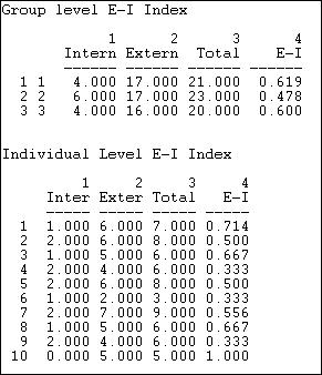
The first panel of figure 8.12 shows the raw counts of ties within and without each of the three types of organizations, and the E-I index for each group. Governmental generalists (group 2) appear to be somewhat more likely to have out-group ties than either of the other sub-populations. The relatively small difference, though, should be treated with considerable caution given the sampling variability (we cannot directly apply the standard error estimate for the whole graph to the results for sub-populations or individuals, but they are suggestive). We should also note that the E-I results for groups and individuals are in "raw" form, and not "rescaled."
There is considerable variability across individuals in their propensity to in-group ties, as can be seen in the last panel of the results. Several actors (4, 6, 9) tend toward closure -- having a preponderance of ties within their own group; a couple others (10, 1) tend toward a preponderance of ties outside their groups.
Embedding of actors in dyads, triads, neighborhoods, clusters, and groups are all ways in which the social structure of a population may display "texture." All of these forms of embedding structures speak to the issue of the "horizontal differentiation" of the population -- separate, but not necessarily ranked or unequal groupings.
A very common form of embedding of actors in structures, though, does involve unequal rankings. Hierarchies, in which individuals or sub-populations are not only differentiated, but also ranked, are extremely common in social life. The degree of hierarchy in a population speaks to the issue of "vertical differentiation."
While we all have an intuitive sense of what it means for a structure to be a hierarchy. Most would agree that structures can be "more or less" hierarchical. It is necessary to be quite precise about the meaning of the term if we are going to build indexes to measure the degree of hierarchy.
Krackhardt (1994) provided an elegant definition of the meaning of hierarchy, and developed measures of each of the four component dimensions of the concept that he identified. Krackhardt defines a pure, "ideal typical" hierarchy as an "out-tree" graph. An out-tree graph is a directed graph in which all points are connected, and all but one node (the "boss") has an in-degree of one. This means that all actors in the graph (except the ultimate "boss") have a single superior node. The simplest "hierarchy" is a directed line graph A to B to C to D... More complex hierarchies may have wider, and varying "spans of control" (out-degrees of points).
This very simple definition of the pure type of hierarchy can be deconstructed into four individually necessary and jointly sufficient conditions. Krackhardt develops index numbers to assess the extent to which each of the four dimensions deviates from the pure ideal type of an out-tree, and hence develops four measures of the extent to which a given structure resembles the ideal typical hierarchy.
1) Connectedness: To be a pure out-tree, a graph must be connected into a single component -- all actors are embedded in the same structure. We can measure the extent to which this is not true by looking at the ratio of the number of pairs in the directed graph that are reachable relative to the number of ordered pairs. That is, what proportion of actors cannot be reached by other actors? Where a graph has multiple components -- multiple un-connected sub-populations -- the proportion not reachable can be high. If all the actors are connected in the same component, if there is a "unitary" structure, the graph is more hierarchical.
2) Hierarchy: To be a pure out-tree, there can be no reciprocated ties. Reciprocal relations between two actors imply equal status, and this denies pure hierarchy. We can assess the degree of deviation from pure hierarchy by counting the number of pairs that have reciprocated ties relative to the number of pairs where there is any tie; that is, what proportion of all tied pairs have reciprocated ties.
3) Efficiency: To be a pure out-tree each node must have an in-degree of one. That is, each actor (except the ultimate boss) has a single boss. This aspect of the idea type is termed "efficiency" because structures with multiple bosses have un-necessary redundant communication of orders from superiors to subordinates. The amount of deviation from this aspect of the pure out-tree can be measured by counting the difference between the actual number of links (minus 1, since the ultimate boss has no boss) and the maximum possible number of links. The bigger the difference, the greater the inefficiency. This dimension then measures the extent to which actors have a "single boss."
4) Least upper bound (LUB): To be a pure out-tree, each pair of actors (except pairs formed between the ultimate boss and others) must have an actor that directs ties to both -- that is, command must be unified. The deviation of a graph from this condition can be measured by counting the numbers of pairs of actors that do not have a common boss relative to the number of pairs that could (which depends on the number of actors and the span of control of the ultimate boss).
The Network>Cohesion>Krackhardt GTD algorithms calculate indexes of each of the four dimensions, where higher scores indicate greater hierarchy. Figure 8.13 shows the results for the Knoke information network.
Figure 8.13. Output of Network>Network Properties>Krackhardt GDT for Knoke information network
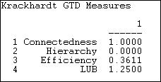
The information network does form a single component, as there is at least one actor that can reach all others. So, the first dimension of pure hierarchy -- that all the actors be embedded in a single structure -- is satisfied. The ties in the information exchange network, though are very likely to be reciprocal (at least insofar as they can be, given the limitations of the density). There are a number of nodes that receive information from multiple others, so the network is not "efficient." The least upper bound measure (the extent to which all actors have a boss in common) reports a value of 1.25, which would appear to be out of range and, frankly, is a puzzle.
This chapter and the next are concerned with the ways in which networks display "structure" or deviation from random connection. In the current chapter, we've approached the same issue of structuring from the "top-down" by looking at patterns of macro-structure in which individuals are embedded in non-random ways. Individuals are embedded (usually simultaneously) in dyads, triads, face-to-face local groups of neighbors, and larger organizational and categorical social structures. The tools in the current chapter provide some ways of examining the "texture" of the structuring of the whole population.
In the next chapter we will focus on the same issue of connection and structure from the "bottom-up." That is, we'll look at structure from the point of view of the individual "ego."
Taken together, the approaches in chapters 8 and 9 illustrate, again, the "duality" of social structure in which individuals make social structures, but do so within a matrix of constraints and opportunities imposed by larger patterns.