Introduction: The several faces of power
All sociologists would agree that power is a fundamental property of social structures. There is much less agreement about what power is, and how we can describe and analyze its causes and consequences. In this chapter we will look at some of the main approaches that social network analysis has developed to study power, and the closely related concept of centrality.
Network thinking has contributed a number of important insights about social power. Perhaps most importantly, the network approach emphasizes that power is inherently relational. An individual does not have power in the abstract, they have power because they can dominate others -- ego's power is alter's dependence. Because power is a consequence of patterns of relations, the amount of power in social structures can vary. If a system is very loosely coupled (low density) not much power can be exerted; in high density systems there is the potential for greater power. Power is both a systemic (macro) and relational (micro) property. The amount of power in a system and its distribution across actors are related, but are not the same thing. Two systems can have the same amount of power, but it can be equally distributed in one and unequally distributed in another. Power in social networks may be viewed either as a micro property (i.e. it describes relations between actors) or as a macro property (i.e. one that describes the entire population); as with other key sociological concepts, the macro and micro are closely connected in social network thinking.
Network analysts often describe the way that an actor is embedded in a relational network as imposing constraints on the actor, and offering the actor opportunities. Actors that face fewer constraints, and have more opportunities than others are in favorable structural positions. Having a favored position means that an actor may extract better bargains in exchanges, have greater influence, and that the actor will be a focus for deference and attention from those in less favored positions.
But, what do we mean by "having a favored position" and having "more opportunities" and "fewer constraints?" There are no single correct and final answers to these difficult questions. But, network analysis has made important contributions in providing precise definitions and concrete measures of several different approaches to the notion of the power that attaches to positions in structures of social relations.
To understand the approaches that network analysis uses to study power, it is useful to first think about some very simple systems. Consider the three simple graphs of networks in figures 10.1, 10.2, and 10.3, which are called the "star," "line," and "circle."
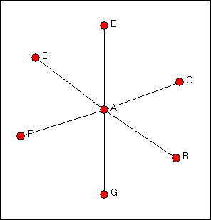
Figure 10.2. "Line" network
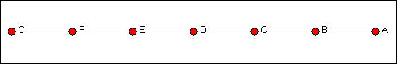
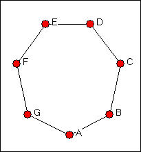
Figure 10.3. "Circle" network
A moment's inspection ought to suggest that actor A has a highly favored structural position in the star network, if the network is describing a relationship such as resource exchange or resource sharing. But, exactly why is it that actor A has a "better" position than all of the others in the star network? What about the position of A in the line network? Is being at the end of the line an advantage or a disadvantage? Are all of the actors in the circle network really in exactly the same structural position?
We need to think about why structural location can be advantageous or disadvantageous to actors. Let's focus our attention on why actor A is so obviously at an advantage in the star network.
Degree: In the star network, actor A has more opportunities and alternatives than other actors. If actor D elects to not provide A with a resource, A has a number of other places to go to get it; however, if D elects to not exchange with A, then D will not be able to exchange at all. The more ties an actor has then, the more power they (may) have. In the star network, Actor A has degree six, all other actors have degree one. This logic underlies measures of centrality and power based on actor degree, which we will discuss below. Actors who have more ties have greater opportunities because they have choices. This autonomy makes them less dependent on any specific other actor, and hence more powerful.
Now, consider the circle network in terms of degree. Each actor has exactly the same number of alternative trading partners (or degree), so all positions are equally advantaged or disadvantaged.
In the line network, matters are a bit more complicated. The actors at the end of the line (A and G) are actually at a structural disadvantage, but all others are apparently equal (actually, it's not really quite that simple). Generally, though, actors that are more central to the structure, in the sense of having higher degree or more connections, tend to have favored positions, and hence more power.
Closeness: The second reason why actor A is more powerful than the other actors in the star network is that actor A is closer to more actors than any other actor. Power can be exerted by direct bargaining and exchange. But power also comes from acting as a "reference point" by which other actors judge themselves, and by being a center of attention who's views are heard by larger numbers of actors. Actors who are able to reach other actors at shorter path lengths, or who are more reachable by other actors at shorter path lengths have favored positions. This structural advantage can be translated into power. In the star network, actor A is at a geodesic distance of one from all other actors; each other actor is at a geodesic distance of two from all other actors (but A). This logic of structural advantage underlies approaches that emphasize the distribution of closeness and distance as a source of power.
Now consider the circle network in terms of actor closeness. Each actor lies at different path lengths from the other actors, but all actors have identical distributions of closeness, and again would appear to be equal in terms of their structural positions. In the line network, the middle actor (D) is closer to all other actors than are the set C,E, the set B,F, and the set A,G. Again, the actors at the ends of the line, or at the periphery, are at a disadvantage.
Betweenness: The third reason that actor A is advantaged in the star network is because actor A lies between each other pairs of actors, and no other actors lie between A and other actors. If A wants to contact F, A may simply do so. If F wants to contact B, they must do so by way of A. This gives actor A the capacity to broker contacts among other actors -- to extract "service charges" and to isolate actors or prevent contacts. The third aspect of a structurally advantaged position then is in being between other actors.
In the circle network, each actor lies between each other pair of actors. Actually, there are two pathways connecting each pair of actors, and each third actor lies on one, but not on the other of them. Again, all actors are equally advantaged or disadvantaged. In the line network, our end points (A,G) do not lie between any pairs, and have no brokering power. Actors closer to the middle of the chain lie on more pathways among pairs, and are again in an advantaged position.
Each of these three ideas -- degree, closeness, and betweenness -- has been elaborated in a number of ways. We will examine three such elaborations briefly here.
Network analysts are more likely to describe their approaches as descriptions of centrality than of power. Each of the three approaches (degree, closeness, betweenness) describe the locations of individuals in terms of how close they are to the "center" of the action in a network -- though the definitions of what it means to be at the center differ. It is more correct to describe network approaches this way -- measures of centrality -- than as measures of power. But, as we have suggested here, there are several reasons why central positions tend to be powerful positions.
Degree centrality
Actors who have more ties to other actors may be advantaged positions. Because they have many ties, they may have alternative ways to satisfy needs, and hence are less dependent on other individuals. Because they have many ties, they may have access to, and be able to call on more of the resources of the network as a whole. Because they have many ties, they are often third-parties and deal makers in exchanges among others, and are able to benefit from this brokerage. So, a very simple, but often very effective measure of an actor's centrality and power potential is their degree.
In undirected data, actors differ from one another only in how many connections they have. With directed data, however, it can be important to distinguish centrality based on in-degree from centrality based on out-degree. If an actor receives many ties, they are often said to be prominent, or to have high prestige. That is, many other actors seek to direct ties to them, and this may indicate their importance. Actors who have unusually high out-degree are actors who are able to exchange with many others, or make many others aware of their views. Actors who display high out-degree centrality are often said to be influential actors.
Recall Knoke's data on information exchanges among organizations operating in the social welfare field, shown in figure 10.1.
Figure 10.4. Knoke's information exchange network
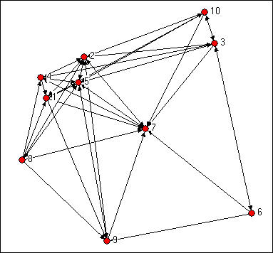
Simply counting the number of in-ties and out-ties of the nodes suggests that certain actors are more "central" here (e.g. 2, 5, 7). It also appears that this network as a whole may have a group of central actors, rather than a single "star." We can see "centrality" as an attribute of individual actors as a consequence of their position; we can also see how "centralized" the graph as a whole is -- how unequal is the distribution of centrality.
Degree centrality: Freeman's approach
Linton Freeman (one of the authors of UCINET) developed basic measures of the centrality of actors based on their degree, and the overall centralization of graphs.
Figure 10.5 shows the output of Network>Centrality>Degree applied to out-degrees and to the in-degrees of the Knoke information network. The centrality can also be computed ignoring the direction of ties (i.e. a tie in either direction is counted as a tie).
Figure 10.5. Freeman degree centrality and graph centralization of Knoke information network
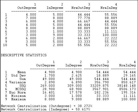
Actors #5 and #2 have the greatest out-degrees, and might be regarded as the most influential (though it might matter to whom they are sending information, this measure does not take that into account). Actors #5 and #2 are joined by #7 (the newspaper) when we examine in-degree. That other organizations share information with these three would seem to indicate a desire on the part of others to exert influence. This is an act of deference, or a recognition that the positions of actors 5, 2, and 7 might be worth trying to influence. If we were interested in comparing across networks of different sizes or densities, it might be useful to "standardize" the measures of in and out-degree. In the last two columns of the first panel of results above, all the degree counts have been expressed as percentages of the number of actors in the network, less one (ego).
The next panel of results speaks to the "meso" level of analysis. That is, what does the distribution of the actor's degree centrality scores look like? On the average, actors have a degree of 4.9, which is quite high, given that there are only nine other actors. We see that the range of in-degree is slightly larger (minimum and maximum) than that of out-degree, and that there is more variability across the actors in in-degree than out-degree (standard deviations and variances). The range and variability of degree (and other network properties) can be quite important, because it describes whether the population is homogeneous or heterogeneous in structural positions. One could examine whether the variability is high or low relative to the typical scores by calculating the coefficient of variation (standard deviation divided by mean, times 100) for in-degree and out-degree. By the rules of thumb that are often used to evaluate coefficients of variation, the current values (35 for out-degree and 53 for in-degree) are moderate. Clearly, however, the population is more homogeneous with regard to out-degree (influence) than with regard to in-degree (prominence).
The last bit of information provided by the output above are Freeman's graph centralization measures, which describe the population as a whole -- the macro level. These are very useful statistics, but require a bit of explanation.
Remember our "star" network from the discussion above (if not, go review it)? The star network is the most centralized or most unequal possible network for any number of actors. In the star network, all the actors but one have degree of one, and the "star" has degree of the number of actors, less one. Freeman felt that it would be useful to express the degree of variability in the degrees of actors in our observed network as a percentage of that in a star network of the same size. This is how the Freeman graph centralization measures can be understood: they express the degree of inequality or variance in our network as a percentage of that of a perfect star network of the same size. In the current case, the out-degree graph centralization is 51% and the in-degree graph centralization 38% of these theoretical maximums. We would arrive at the conclusion that there is a substantial amount of concentration or centralization in this whole network. That is, the power of individual actors varies rather substantially, and this means that, overall, positional advantages are rather unequally distributed in this network.
Degree centrality: Bonacich's approach
Phillip Bonacich proposed a modification of the degree centrality approach that has been widely accepted as superior to the original measure. Bonacich's idea, like most good ones, is pretty simple. The original degree centrality approach argues that actors who have more connections are more likely to be powerful because they can directly affect more other actors. This makes sense, but having the same degree does not necessarily make actors equally important.
Suppose that Bill and Fred each have five close friends. Bill's friends, however, happen to be pretty isolated folks, and don't have many other friends, save Bill. In contrast, Fred's friends each also have lots of friends, who have lots of friends, and so on. Who is more central? We would probably agree that Fred is, because the people he is connected to are better connected than Bill's people. Bonacich argued that one's centrality is a function of how many connections one has, and how many the connections the actors in the neighborhood had.
While we have argued that more central actors are more likely to be more powerful actors, Bonacich questioned this idea. Compare Bill and Fred again. Fred is clearly more central, but is he more powerful? One argument would be that one is likely to be more influential if one is connected to central others -- because one can quickly reach a lot of other actors with one's message. But if the actors that you are connected to are, themselves, well connected, they are not highly dependent on you -- they have many contacts, just as you do. If, on the other hand, the people to whom you are connected are not, themselves, well connected, then they are dependent on you. Bonacich argued that being connected to connected others makes an actor central, but not powerful. Somewhat ironically, being connected to others that are not well connected makes one powerful, because these other actors are dependent on you -- whereas well connected actors are not.
Bonacich proposed that both centrality and power were a function of the connections of the actors in one's neighborhood. The more connections the actors in your neighborhood have, the more central you are. The fewer the connections the actors in your neighborhood, the more powerful you are. There would seem to be a problem with building an algorithms to capture these ideas. Suppose A and B are connected. Actor A's power and centrality are functions of her own connections, and also the connections of actor B. Similarly, actor B's power and centrality depend on actor A's. So, each actor's power and centrality depends on each other actor's power simultaneously.
There is a way out of this chicken-and-egg type of problem. Bonacich showed that, for symmetric systems, an iterative estimation approach to solving this simultaneous equations problem would eventually converge to a single answer. One begins by giving each actor an estimated centrality equal to their own degree, plus a weighted function of the degrees of the actors to whom they were connected. Then, we do this again, using the first estimates (i.e. we again give each actor an estimated centrality equal to their own first score plus the first scores of those to whom they are connected). As we do this numerous times, the relative sizes (not the absolute sizes) of all actors scores will come to be the same. The scores can then be re-expressed by scaling by constants.
Let's examine the centrality and power scores for our information exchange data. First, we examine the case where the score for each actor is a positive function of their own degree, and the degrees of the others to whom they are connected. We do this by selecting a positive weight of the "attenuation factor" or Beta parameter) in the dialog of Network>Centrality>Power, as shown in figure 10.6.
Figure 10.6. Dialog for computing Bonacich's power measures
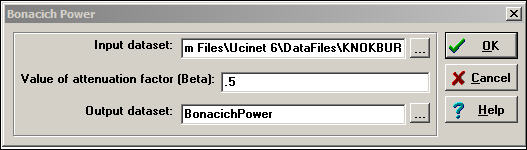
The "attenuation factor" indicates the effect of one's neighbor's connections on ego's power. Where the attenuation factor is positive (between zero and one), being connected to neighbors with more connections makes one powerful. This is a straight-forward extension of the degree centrality idea.
Bonacich also had a second idea about power, based on the notion of "dependency." If ego has neighbors who do not have many connections to others, those neighbors are likely to be dependent on ego, making ego more powerful. Negative values of the attenuation factor (between zero and negative one) compute power based on this idea.
Figures 10.7 and 10.8 show the Bonacich measures for positive and negative beta values.
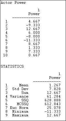
Figure 10.7. Network>Centrality>Power with beta = + .50
If we look at the absolute value of the index scores, we see the familiar story. Actors #5 and #2 are clearly the most central. This is because they have high degree, and because they are connected to each other, and to other actors with high degree. Actors 8 and 10 also appear to have high centrality by this measure -- this is a new result. In these case, it is because the actors are connected to all of the other high degree points. These actors don't have extraordinary numbers of connections, but they have "the right connections."
Let's take a look at the power side of the index, which is calculated by the same algorithm, but gives negative weights to connections with well connected others, and positive weights for connections to weakly connected others.
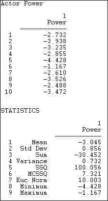
Figure 10.8. Network>Centrality>Power with beta = - .50
Not surprisingly, these results are very different from many of the others we've examined. With a negative attenuation parameter, we have a quite different definition of power -- having weak neighbors, rather than strong ones. Actors numbers 2 and 6 are distinguished because their ties are mostly ties to actors with high degree -- making actors 2 and 6 "weak" by having powerful neighbors. Actors 3, 7, and 9 have more ties to neighbors who have few ties -- making them "strong" by having weak neighbors. You might want to scan the diagram again to see if you can see these differences.
The Bonacich approach to degree based centrality and degree based power are fairly natural extensions of the idea of degree centrality based on adjacencies. One is simply taking into account the connections of one's connections, in addition to one's own connections. The notion that power arises from connection to weak others, as opposed to strong others is an interesting one, and points to yet another way in which the positions of actors in network structures endow them with different potentials.
Closeness centrality
Degree centrality measures might be criticized because they only take into account the immediate ties that an actor has, or the ties of the actor's neighbors, rather than indirect ties to all others. One actor might be tied to a large number of others, but those others might be rather disconnected from the network as a whole. In a case like this, the actor could be quite central, but only in a local neighborhood.
Closeness centrality approaches emphasize the distance of an actor to all others in the network by focusing on the distance from each actor to all others. Depending on how one wants to think of what it means to be "close" to others, a number of slightly different measures can be defined.
Path distances
Network>Centrality>Closeness provides a number of alternative ways of calculating the "far-ness" of each actor from all others. Far-ness is the sum of the distance (by various approaches) from each ego to all others in the network.
"Far-ness" is then transformed into "nearness" as the reciprocal of farness. That is, nearness = one divided by farness. "Nearness" can be further standardized by norming against the minimum possible nearness for a graph of the same size and connection.
Given a measure of nearness or farness for each actor, we can again calculate a measure of inequality in the distribution of distances across the actors, and express "graph centralization" relative to that of the idealized "star" network.
Figure 10.9 shows a dialog for calculating closeness measures of centrality and graph centralization.
Figure 10.9. Dialog for Network>Centrality>Closeness
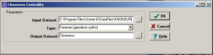
Several alternative approaches to measuring "far-ness" are available in the type setting. The most common is probably the geodesic path distance. Here, "far-ness" is the sum of the lengths of the shortest paths from ego (or to ego) from all other nodes. Alternatively, the reciprocal of this, or "near-ness" can be calculated. Alternatively, one may focus on all paths, not just geodesics, or all trails. Figure 10.10 shows the results for the Freeman geodesic path approach.
Figure 10.10. Geodesic path closeness centrality for Knoke information network
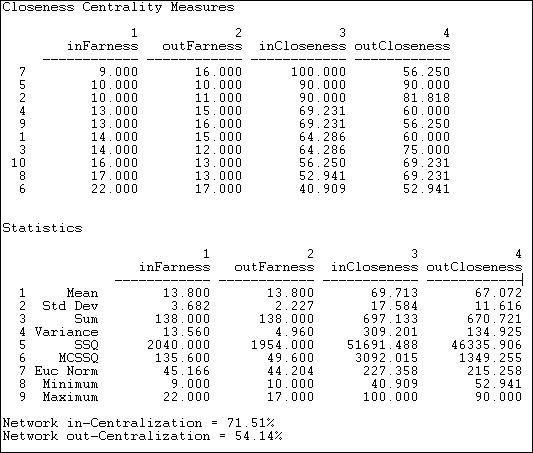
Since the information network is directed, separate close-ness and far-ness can be computed for sending and receiving. We see that actor 6 has the largest sum of geodesic distances from other actors (inFarness of 22) and to other actors (outFarness of 17). The farness figures can be re-expressed as nearness (the reciprocal of far-ness) and normed relative to the greatest nearness observed in the graph (here, the inCloseness of actor 7).
Summary statistics on the distribution of the nearness and farness measures are also calculated. We see that the distribution of out-closeness has less variability than in-closeness, for example. This is also reflected in the graph in-centralization (71.5%) and out-centralization (54.1%) measures; that is, in-distances are more un-equally distributed than are out-distances.
Closeness: Reach
Another way of thinking about how close an actor is to all others is to ask what portion of all others ego can reach in one step, two steps, three steps, etc. The routine Network>Centrality>Reach Centrality calculates some useful measures of how close each actor is to all others. Figure 10.11 shows the results for the Knoke information network.
Figure 10.11. Reach centrality for Knoke information network
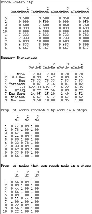
An index of the "reach distance" from each ego to (or from) all others is calculated. Here, the maximum score (equal to the number of nodes) is achieved when every other is one-step from ego. The reach closeness sum becomes less as actors are two steps, three steps, and so on (weights of 1/2, 1/3, etc.). These scores are then expressed in "normed" form by dividing by the largest observed reach value.
The final two tables are quite easy to interpret. The first of these shows what proportion of other nodes can be reached from each actor at one, two, and three steps (in our example, all others are reachable in three steps or less). The last table shows what proportions of others can reach ego at one, two, and three steps. Note that everyone can contact the newspaper (actor 7) in one step.
Closeness: Eigenvector of geodesic distances
The closeness centrality measure described above is based on the sum of the geodesic distances from each actor to all others (farness). In larger and more complex networks than the example we've been considering, it is possible to be somewhat misled by this measure. Consider two actors, A and B. Actor A is quite close to a small and fairly closed group within a larger network, and rather distant from many of the members of the population. Actor B is at a moderate distance from all of the members of the population. The farness measures for actor A and actor B could be quite similar in magnitude. In a sense, however, actor B is really more "central" than actor A in this example, because B is able to reach more of the network with same amount of effort.
The eigenvector approach is an effort to find the most central actors (i.e. those with the smallest farness from others) in terms of the "global" or "overall" structure of the network, and to pay less attention to patterns that are more "local." The method used to do this (factor analysis) is beyond the scope of the current text. In a general way, what factor analysis does is to identify "dimensions" of the distances among actors. The location of each actor with respect to each dimension is called an "eigenvalue," and the collection of such values is called the "eigenvector." Usually, the first dimension captures the "global" aspects of distances among actors; second and further dimensions capture more specific and local sub-structures.
The UCINET Network>Centrality>Eigenvector routine calculates individual actor centrality, and graph centralization using weights on the first eigenvector. A limitation of the routine is that it does not calculate values for asymmetric data. So, our measures here are based on the notion of "any connection."
Figure 10.12. Eigenvector centrality and centralization for Knoke information network
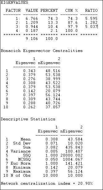
The first set of statistics, the eigenvalues, tell us how much of the overall pattern of distances among actors can be seen as reflecting the global pattern (the first eigenvalue), and more local, or additional patterns. We are interested in the percentage of the overall variation in distances that is accounted for by the first factor. Here, this percentage is 74.3%. This means that about 3/4 of all of the distances among actors are reflective of the main dimension or pattern. If this amount is not large (say over 70%), great caution should be exercised in interpreting the further results, because the dominant pattern is not doing a very complete job of describing the data. The first eigenvalue should also be considerably larger than the second (here, the ratio of the first eigenvalue to the second is about 5.6 to 1). This means that the dominant pattern is, in a sense, 5.6 times as "important" as the secondary pattern.
Next, we turn our attention to the scores of each of the cases on the 1st eigenvector. Higher scores indicate that actors are "more central" to the main pattern of distances among all of the actors, lower values indicate that actors are more peripheral. The results are very similar to those for our earlier analysis of closeness centrality, with actors #7, #5, and #2 being most central, and actor #6 being most peripheral. Usually the eigenvalue approach will do what it is supposed to do: give us a "cleaned-up" version of the closeness centrality measures, as it does here. It is a good idea to examine both, and to compare them.
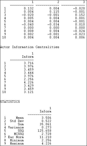
Last, we examine the overall centralization of the graph, and the distribution of centralities. There is relatively little variability in centralities (standard deviation .07) around the mean (.31). This suggests that, overall, there are not great inequalities in actor centrality or power, when measured in this way. Compared to the pure "star" network, the degree of inequality or concentration of the Knoke data is only 20.9% of the maximum possible. This is much less than the network centralization measure for the "raw" closeness measure (49.3), and suggests that some of the apparent differences in power using the raw closeness approach may be due more to local than to global inequalities.
Geodesic distances among actors are a reasonable measure of one
aspect of centrality -- or positional advantage. Sometimes these advantages may be more local, and sometimes more
global. The factor-analytic approach is one approach that may sometimes help us to focus on the more global pattern.
Again, it is not that one approach is "right" and the other "wrong." Depending on the goals
of our analysis, we may wish to emphasize one or the other aspects of the positional advantages that arise from
centrality.
table of contents
Closeness: Hubbell, Katz, Taylor, Stephenson and Zelen influence measures
The geodesic closeness and eigenvalue approaches consider the closeness of connection to all other actors, but only by the "most efficient" path (the geodesic). In some cases, power or influence may be expressed through all of the pathways that connect an actor to all others. Several measures of closeness based on all connections of ego to others are available from Network>Centrality>Influence.
Even if we want to include all connections between two actors, it may not make a great deal of sense to consider a path of length 10 as important as a path of length 1. The Hubbell and Katz approaches count the total connections between actors (ties for undirected data, both sending and receiving ties for directed data). Each connection, however, is given a weight, according to its length. The greater the length, the weaker the connection. How much weaker the connection becomes with increasing length depends on an "attenuation" factor. In our example, below, we have used an attenuation factor of .5. That is, an adjacency receives a weight of one, a walk of length two receives a weight of .5, a connection of length three receives a weight of .5 squared (.25) etc. The Hubbell and Katz approaches are very similar. Katz includes an identity matrix (a connection of each actor with itself) as the strongest connection; the Hubbell approach does not. As calculated by UCINET, both approaches "norm" the results to range from large negative distances (that is, the actors are very close relative to the other pairs, or have high cohesion) to large positive numbers (that is, the actors have large distance relative to others). The results of the Hubbell and Katz approaches are shown in figure 10.13 and 10.14.
Figure 10.13. Hubbell dyadic influence for the Knoke information network
Method:  HUBBELL
               1      2      3      4      5      6      7      8      9     10
            COUN   COMM   EDUC   INDU   MAYR    WRO   NEWS   UWAY   WELF   WEST
          ------ ------ ------ ------ ------ ------ ------ ------ ------ ------
  1 COUN   -0.67  -0.67   2.00  -0.33  -0.67   2.00   0.33  -1.33  -1.33   1.33
  2 COMM   -0.92  -0.17   1.50  -0.08  -0.67   1.50   0.08  -0.83  -1.08   0.83
  3 EDUC    5.83   3.33 -11.00   0.17   3.33 -11.00  -2.17   6.67   8.17  -7.67
  4 INDU   -1.50  -1.00   3.00   0.50  -1.00   3.00   0.50  -2.00  -2.50   2.00
  5 MAYR    1.25   0.50  -2.50  -0.25   1.00  -2.50  -0.75   1.50   1.75  -1.50
  6  WRO    3.83   2.33  -8.00   0.17   2.33  -7.00  -1.17   4.67   6.17  -5.67
  7 NEWS   -1.17  -0.67   2.00   0.17  -0.67   2.00   0.83  -1.33  -1.83   1.33
  8 UWAY   -3.83  -2.33   7.00  -0.17  -2.33   7.00   1.17  -3.67  -5.17   4.67
  9 WELF   -0.83  -0.33   1.00  -0.17  -0.33   1.00   0.17  -0.67  -0.17   0.67
 10 WEST    4.33   2.33  -8.00  -0.33   2.33  -8.00  -1.67   4.67   5.67  -4.67
Figure 10.14. Katz dyadic influence for the Knoke information network
Method:                  KATZ
               1      2      3      4      5      6      7      8      9     10
            COUN   COMM   EDUC   INDU   MAYR    WRO   NEWS   UWAY   WELF   WEST
          ------ ------ ------ ------ ------ ------ ------ ------ ------ ------
  1 COUN   -1.67  -0.67   2.00  -0.33  -0.67   2.00   0.33  -1.33  -1.33   1.33
  2 COMM   -0.92  -1.17   1.50  -0.08  -0.67   1.50   0.08  -0.83  -1.08   0.83
  3 EDUC    5.83   3.33 -12.00   0.17   3.33 -11.00  -2.17   6.67   8.17  -7.67
  4 INDU   -1.50  -1.00   3.00  -0.50  -1.00   3.00   0.50  -2.00  -2.50   2.00
  5 MAYR    1.25   0.50  -2.50  -0.25   0.00  -2.50  -0.75   1.50   1.75  -1.50
  6  WRO    3.83   2.33  -8.00   0.17   2.33  -8.00  -1.17   4.67   6.17  -5.67
  7 NEWS   -1.17  -0.67   2.00   0.17  -0.67   2.00  -0.17  -1.33  -1.83   1.33
  8 UWAY   -3.83  -2.33   7.00  -0.17  -2.33   7.00   1.17  -4.67  -5.17   4.67
  9 WELF   -0.83  -0.33   1.00  -0.17  -0.33   1.00   0.17  -0.67  -1.17   0.67
 10 WEST    4.33   2.33  -8.00  -0.33   2.33  -8.00  -1.67   4.67   5.67  -5.67
As with all measures of pair-wise properties, one could analyze the data much further. We could see which individuals are similar to which others (that is, are there groups or strata defined by the similarity of their total connections to all others in the network?). Our interest might also focus on the whole network, where we might examine the degree of variance, and the shape of the distribution of the dyads connections. For example, a network in with the total connections among all pairs of actors might be expected to behave very differently than one where there are radical differences among actors.
The Hubbell and Katz approach may make most sense when applied to symmetric data, because they pay no attention to the directions of connections (i.e. A's ties directed to B are just as important as B's ties to A in defining the distance or solidarity -- closeness-- between them). If we are more specifically interested in the influence of A on B in a directed graph, the Taylor influence approach provides an interesting alternative.
The Taylor measure, like the others, uses all connections, and applies an attenuation factor. Rather than standardizing on the whole resulting matrix, however, a different approach is adopted. The column marginals for each actor are subtracted from the row marginals, and the result is then normed (what did he say?!). Translated into English, we look at the balance between each actors sending connections (row marginals) and their receiving connections (column marginals). Positive values then reflect a preponderance of sending over receiving to the other actor of the pair -- or a balance of influence between the two. Note that the newspaper (#7) shows as being a net influencer with respect to most other actors in the result below, while the welfare rights organization (#6) has a negative balance of influence with most other actors. The results for the Knoke information network are shown in figure 10.15.
Figure 10.15. Taylor dyadic influence for the Knoke information network
Method: TAYLOR
              1     2     3     4     5     6     7     8     9    10
           COUN  COMM  EDUC  INDU  MAYR   WRO  NEWS  UWAY  WELF  WEST
          ----- ----- ----- ----- ----- ----- ----- ----- ----- -----
  1 COUN   0.00 -0.02  0.23 -0.07  0.12  0.11 -0.09 -0.15  0.03  0.18
  2 COMM   0.02  0.00  0.11 -0.06  0.07  0.05 -0.05 -0.09  0.05  0.09
  3 EDUC  -0.23 -0.11  0.00  0.17 -0.36  0.18  0.26  0.02 -0.44 -0.02
  4 INDU   0.07  0.06 -0.17  0.00  0.05 -0.17 -0.02  0.11  0.14 -0.14
  5 MAYR  -0.12 -0.07  0.36 -0.05  0.00  0.30  0.01 -0.23 -0.13  0.23
  6  WRO  -0.11 -0.05 -0.18  0.17 -0.30  0.00  0.19  0.14 -0.32 -0.14
  7 NEWS   0.09  0.05 -0.26  0.02 -0.01 -0.19  0.00  0.15  0.12 -0.18
  8 UWAY   0.15  0.09 -0.02 -0.11  0.23 -0.14 -0.15  0.00  0.28  0.00
  9 WELF  -0.03 -0.05  0.44 -0.14  0.13  0.32 -0.12 -0.28  0.00  0.31
 10 WEST  -0.18 -0.09  0.02  0.14 -0.23  0.14  0.18 -0.00 -0.31  0.00
Yet another measure based on attenuating and norming all pathways between each actor and all others was proposed by Stephenson and Zelen, and can be computed with Network>Centrality>Information. This measure, shown in figure 10.16, provides a more complex norming of the distances from each actor to each other, and summarizes the centrality of each actor with the harmonic mean of its distance to the others.
Figure 10.16. Stephenson and Zelen information centrality of Knoke information network
The (truncated) top panel shows the dyadic distance of each actor to each other. The summary measure is shown in the middle panel, and information about the distribution of the centrality scores is shown in the statistics section.
As with most other measures, the various approaches to the distance between actors and in the network as a whole provide a menu of choices. No one definition to measuring distance will be the "right" choice for a given purpose. Sometimes we don't really know, before hand, what approach might be best, and we may have to try and test several.
Betweenness centrality
Suppose that I want to influence you by sending you information, or make a deal to exchange some resources. But, in order to talk to you, I must go through an intermediary. For example, let's suppose that I wanted to try to convince the Chancellor of my university to buy me a new computer. According to the rules of our bureaucratic hierarchy, I must forward my request through my department chair, a dean, and an executive vice chancellor. Each one of these people could delay the request, or even prevent my request from getting through. This gives the people who lie "between" me and the Chancellor power with respect to me. To stretch the example just a bit more, suppose that I also have an appointment in the school of business, as well as one in the department of sociology. I might forward my request to the Chancellor by both channels. Having more than one channel makes me less dependent, and, in a sense, more powerful.
For networks with binary relations, Freeman created some measures of the centrality of individual actors based on their betweenness, as well overall graph centralization. Freeman, Borgatti, and White extended the basic approach to deal with valued relations.
Betweenness: Freeman's approach to binary relations
With binary data, betweenness centrality views an actor as being in a favored position to the extent that the actor falls on the geodesic paths between other pairs of actors in the network. That is, the more people depend on me to make connections with other people, the more power I have. If, however, two actors are connected by more than one geodesic path, and I am not on all of them, I lose some power. Using the computer, it is quite easy to locate the geodesic paths between all pairs of actors, and to count up how frequently each actor falls in each of these pathways. If we add up, for each actor, the proportion of times that they are "between" other actors for the sending of information in the Knoke data, we get the a measure of actor centrality. We can norm this measure by expressing it as a percentage of the maximum possible betweenness that an actor could have had. Network>Centrality>Betweenness>Nodes can be used to calculate Freeman's betweenness measures for actors. The results for the Knoke information network are shown in figure 10.17.
Figure 10.17. Freeman node betweenness for Knoke information network
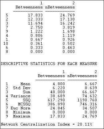
We can see that there is a lot of variation in actor betweenness (from zero to 17.83), and that there is quite a bit of variation (std. dev. = 6.2 relative to a mean betweenness of 4.8). Despite this, the overall network centralization is relatively low. This makes sense, because we know that fully one half of all connections can be made in this network without the aid of any intermediary -- hence there cannot be a lot of "betweenness." In the sense of structural constraint, there is not a lot of "power" in this network. Actors #2, #3, and #5 appear to be relatively a good bit more powerful than others by this measure. Clearly, there is a structural basis for these actors to perceive that they are "different" from others in the population. Indeed, it would not be surprising if these three actors saw themselves as the movers-and-shakers, and the deal-makers that made things happen. In this sense, even though there is not very much betweenness power in the system, it could be important for group formation and stratification.
Another way to think about betweenness is to ask which relations are most central, rather than which actors. Freeman's definition can be easily applied: a relation is between to the extent that it is part of the geodesic between pairs of actors. Using this idea, we can calculate a measure of the extent to which each relation in a binary graph is between. In UCINET, this is done with Network>Centrality>Betweenness>Lines (edges). The results for the Knoke information network are shown in figure 10.18.
Figure 10.18. Freeman edge betweenness for Knoke information network
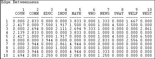
A number of the relations (or potential relations) between pairs of actors are not parts of any geodesic paths (e.g. the relation from actor 1 to actor 3). Betweenness is zero if there is no tie, or if a tie that is present is not part of any geodesic paths. There are some quite central relations in the graph. For example, the tie from the board of education (actor 3) to the welfare rights organization (actor 6). This particular high value arises because without the tie to actor 3, actor 6 would be largely isolated.
Suppose A has ties to B and C. B has ties to D and E; C has ties to F and G. Actor "A" will have high betweenness, because it connects two branches of ties, and lies on many geodesic paths. Actors B and C also have betweenness, because they lie between A and their "subordinates." But actors D, E, F, and G have zero betweenness.
One way of identifying hierarchy in a set of relations is to locate the "subordinates." These actors will be ones with no betweenness. If we then remove these actors from the graph, some of the remaining actors won't be between any more -- so they are one step up in the hierarchy. We can continue doing this "hierarchical reduction" until we've exhausted the graph; what we're left with is a map of the levels of the hierarchy.
Network>Centrality>Betweenness>Hierarchical Reduction is an algorithm that identifies which actors fall at which levels of a hierarchy (if there is one). Since there is very little hierarchy in the Knoke data, we've illustrated this instead with a network of large donors to political campaigns in California, who are "connected" if they contribute to the same campaign. A part of the results is shown in figure 10.19.
Figure 10.19. Hierarchical reduction by betweenness for California political donors (truncated)
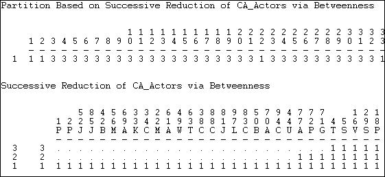
In these data, it turns out that a three-level hierarchy can be identified. The first portion of the output shows a partition (which can be saved as a file, and used as an attribute to color a graph) of the node's level in the hierarchy. The first two nodes, for example, are at the lowest level (1) of the hierarchy, while the third node is at the third level. The second portion of the output has re-arranged the nodes to show which actors are included at the lowest betweenness (level one, or everyone); which drop out at level 2 (that is, are most subordinate, e.g. actors 1, 2, 52); and successive levels. Our data has a hierarchical depth of only three.
Betweenness: Flow centrality
The betweenness centrality measure we examined above characterizes actors as having positional advantage, or power, to the extent that they fall on the shortest (geodesic) pathway between other pairs of actors. The idea is that actors who are "between" other actors, and on whom other actors must depend to conduct exchanges, will be able to translate this broker role into power.
Suppose that two actors want to have a relationship, but the geodesic path between them is blocked by a reluctant broker. If there exists another pathway, the two actors are likely to use it, even if it is longer and "less efficient." In general, actors may use all of the pathways connecting them, rather than just geodesic paths. The flow approach to centrality expands the notion of betweenness centrality. It assumes that actors will use all pathways that connect them, proportionally to the length of the pathways. Betweenness is measured by the proportion of the entire flow between two actors (that is, through all of the pathways connecting them) that occurs on paths of which a given actor is a part. For each actor, then, the measure adds up how involved that actor is in all of the flows between all other pairs of actors (the amount of computation with more than a couple actors can be pretty intimidating!). Since the magnitude of this index number would be expected to increase with sheer size of the network and with network density, it is useful to standardize it by calculating the flow betweenness of each actor in ratio to the total flow betweenness that does not involve the actor.
The algorithm Network>Centrality>Flow Betweenness calculates actor and graph flow betweenness centrality measures. Results of applying this to the Knoke information network are shown in figure 10.20.
Figure 10.20. Flow betweenness centrality for Knoke information network
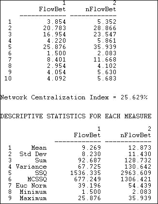
By this more complete measure of betweenness centrality, actors #2 and #5 are clearly the most important mediators. Actor #3, who was fairly important when we considered only geodesic flows, appears to be rather less important. While the overall picture does not change a great deal, the elaborated definition of betweenness does give us a somewhat different impression of who is most central in this network.
Some actors are clearly more central than others, and the relative variability in flow betweenness of the actors is fairly great (the standard deviation of normed flow betweenness is 8.2 relative to a mean of 9.2, giving a coefficient of relative variation). Despite this relatively high amount of variation, the degree of inequality, or concentration in the distribution of flow betweenness centralities among the actors is fairly low -- relative to that of a pure star network (the network centralization index is 25.6%). This is slightly higher than the index for the betweenness measure that was based only on geodesic distances.
Summary
Social network analysis methods provide some useful tools for addressing one of the most important (but also one of the most complex and difficult), aspects of social structure: the sources and distribution of power. The network perspective suggests that the power of individual actors is not an individual attribute, but arises from their relations with others. Whole social structures may also be seen as displaying high levels or low levels of power as a result of variations in the patterns of ties among actors. And, the degree of inequality or concentration of power in a population may be indexed.
Power arises from occupying advantageous positions in networks of relations. Three basic sources of advantage are high degree, high closeness, and high betweenness. In simple structures (such as the star, circle, or line), these advantages tend to covary. In more complex and larger networks, there can be considerable disjuncture between these characteristics of a position-- so that an actor may be located in a position that is advantageous in some ways, and disadvantageous in others.
We have reviewed three basic approaches to the "centrality" of individuals positions, and some elaborations on each of the three main ideas of degree, closeness, and betweenness. This review is not exhaustive. The question of how structural position confers power remains a topic of active research and considerable debate. As you can see, different definitions and measures can capture different ideas about where power comes from, and can result in some rather different insights about social structures.
In the last chapter and this one, we have emphasized that social network analysis methods give us, at the same time, views of individuals and of whole populations. One of the most enduring and important themes in the study of human social organization, however, is the importance of social units that lie between the the two poles of individuals and whole populations. In the next chapter, we will turn our attention to how network analysis methods describe and measure the differentiation of sub-populations.
Review Questions
1. What is the difference between "centrality" and "centralization?"
2. Why is an actor who has higher degree a more "central" actor?
3. How does Bonacich's influence measure extend the idea of degree centrality?
4. Can you explain why an actor who has the smallest sum of geodesic distances to all other actors is said to be the most "central" actor, using the "closeness" approach?
5. How does the "flow" approach extend the idea of "closeness" as an approach to centrality?
6. What does it mean to say that an actor lies "between" two other actors? Why does betweenness give an actor power or influence?
7. How does the "flow" approach extend the idea of "betweenness" as an approach to centrality?
8. Most approaches suggest that centrality confers power and influence. Bonacich suggests that power and influence are not the same thing. What is Bonacich' arguement? How does Bonacich measure the power of an actor?
Application Questions
1. Think of the readings from the first part of the course. Which studies used the ideas of structural advantage, centrality, power and influence? What kinds of approach did each use: degree, closeness, or betweenness?
2. Can you think of any circumstances where being "central" might make one less influential? less powerful?
3. Consider a directed network that describes a hierarchical bureaucracy, where the relationship is "gives orders to." Which actors have highest degree? are they the most powerful and influential? Which actors have high closeness? Which actors have high betweenness?
4. Can you think of a real-world example of an actor who might be powerful but not central? who might be central, but not powerful?
table of contents
table of contents of the book